Developing machine learning (ML) techniques for complex, real-world materials poses challenges which are not commonly encountered in traditional machine learning research. The most critical of these is the size of available datasets, and the distribution of data points therein. While traditional ML algorithms work best with tens or even hundreds of thousands of samples, and modern large language models are trained on datasets encompassing more or less the entire internet, the size of high-quality experimental datasets for industrial materials is usually measured in the hundreds. In addition, some material classes, such as ferrous or aluminium alloys, have been much more extensively investigated than others.
The very fact that experimental measurements are often time-consuming and difficult to carry out, however, makes the design and characterisation of novel materials for high-tech applications, such as in NICKEFFECT, a tempting target for ML. It is therefore necessary to develop techniques with which to train high-quality models on small datasets. One such approach can be summarised as “knowing what you don’t know”, or, more formally, uncertainty quantification.
Uncertainty quantification approaches require the ML model to predict not just the property itself, such as the current carried by a material, but also how confident it is in the prediction. In materials science, a particularly popular technique for achieving this is ensembling, where several models are trained under slightly different conditions, such as using different model architectures or different data subsets. The standard deviation of the separate models’ predictions can then be used as the uncertainty:
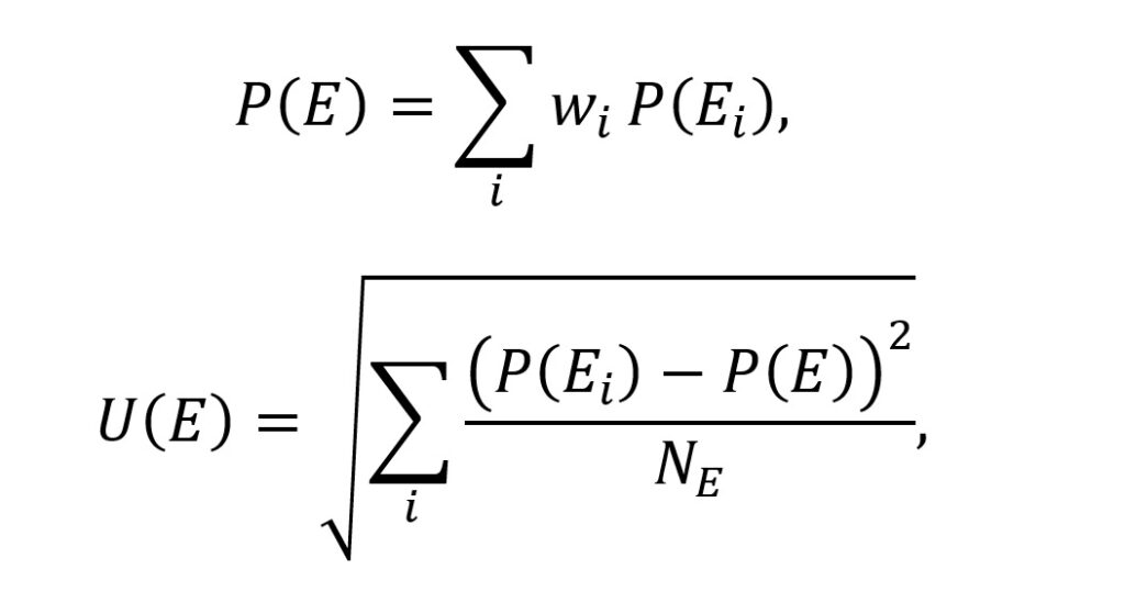
Where P is a prediction, E is the ensemble, Ei is one of the models in the ensemble, NE is the total number of models constituting the ensemble, and U is the uncertainty.
Uncertainty quantification is a non-trivial task – heuristically this can be understood by considering that if the error itself could be predicted, a sufficiently powerful model would learn this and predict the relevant property more accurately in the first place! It is therefore critical to verify that a model’s uncertainty correlates with the real error. The relationship between the two can be visualised in an ‘uncertainty parity curve’:
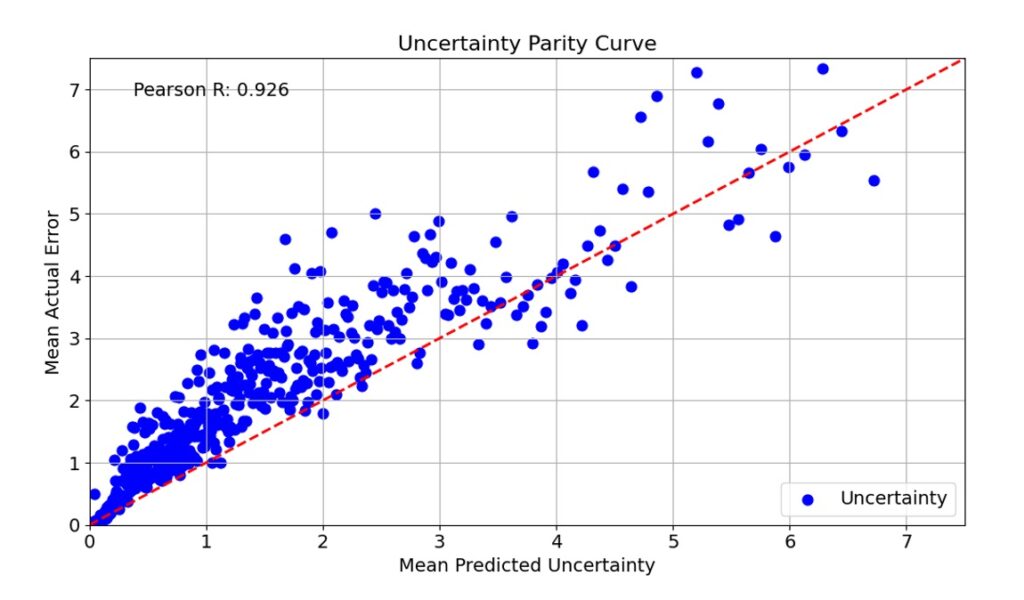
In this example, we see that, while the relation between uncertainty and error is certainly noisy, the trend is very well-captured. As a result, high uncertainties tend to be predictive of high errors, which makes the uncertainty suitable for postprocessing tasks aiming to improve the prediction. For instance, it can be used to indicate uncertainty regions in plots of materials properties vs temperature:
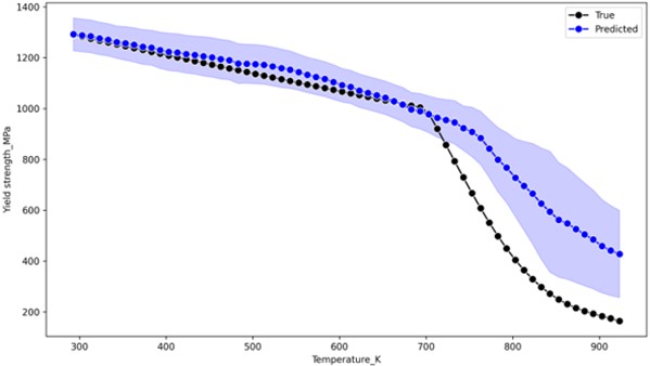
Here, the uncertain high-temperature region corresponds to a regime in which our prediction is notably worse than the excellent quality achieved at lower temperatures.
In addition to active learning (covered in a previous blog post), the uncertainty can also be used to enable the model to refuse to predict in highly uncertain regimes, giving user more confidence in those regimes where the model does make a prediction.
The performance improvement which can be obtained by these means can be estimated using the “sparsification curve”, charting how much the prediction error on a testing set is reduced when removing the x% most uncertain predictions:
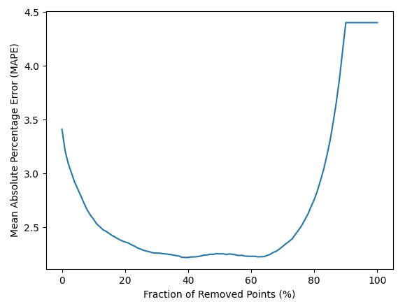
In this case, we see rapid error reduction up to a removal fraction of ~20%, after which point the improvement decelerates, until levelling out completely at ~40%. At its optimal point, we can expect an improvement of more than one third from the removal of uncertain points. When more than ~70% of data is removed, the error begins to increase quickly!
The sparsification curve’s behaviour reflects our previous insight that uncertainty quantification methods cannot possibly be perfect – at a certain point, the next prediction you remove is as likely to be better as it is to be worse than the average. If perfect error prediction were possible, the error would decline all the way to 0 as we approach a 100% approval fraction.
Even in absence of such an ‘oracle’, uncertainty quantification is a powerful addition to the ML toolkit. In practice, when deciding how many points to remove, we will have to balance the partially contradictory objectives of maximum error reduction and maximum prediction retention. In the above case, for instance, we might settle for refusing to predict the property when its model uncertainty is among the top 15% of uncertainty values. This would retain a large amount of predictive capacity while reducing the error by more than 25%. Furthermore, uncertainty quantification is only one example of how we have tackled the challenge of materials ML. It can be combined with other approaches, for instance embedding of physical knowledge in the model, to achieve further improvements. In this manner, relatively simple statistical techniques can enable high-accuracy predictive modelling of industrial materials and unlock real-world impact even with comparatively small datasets.
